September 2023 I Volume 44, Issue 3
Development of Wald-Type and Score-Type Statistical Tests to Compare Live Test Data and Simulation Predictions
September 2023
Volume 44 I Issue 3
![]()
IN THIS JOURNAL:
- Issue at a Glance
- Chairman’s Message
Conversations with Experts
- Interview with Robert J. Arnold
Technical Articles
- I-TREE A Tool for Characterizing Research Using Taxonomies
- Scientific Measurement of Situation Awareness in Operational Testing
- Using ChangePoint Detection and AI to classify fuel pressure states in Aerial Refueling
- Post-hoc Uncertainty Quantification of Deep Learning Models Applied to Remote Sensing Image Scene Classification
- Development of Wald-Type and Score-Type Statistical Tests to Compare Live Test Data and Simulation Predictions
- Test and Evaluation of Systems with Embedded Machine Learning Components
- Experimental Design for Operational Utility
- Review of Surrogate Strategies and Regularization with Application to High-Speed Flows
- Estimating Sparsely and Irregularly Observed Multivariate Functional Data
- Statistical Methods Development Work for M and S Validation
News
- Association News
- Chapter News
- Corporate Member News
Development of Wald-Type and Score-Type Statistical Tests to Compare Live Test Data and Simulation Predictions

Carrington A. Metts
Data Science Fellow at IDA
![]()
![]()

Curtis Miller, PhD
Research Staff Member of the Operational Evaluation Division at IDA
![]()
![]()
Abstract
This work describes the development of a statistical test created in support of ongoing verification, validation, and accreditation (VV&A) efforts for modeling and simulation (M&S) environments. The test computes a Wald-type statistic comparing two generalized linear models estimated from live test data and analogous simulated data. The resulting statistic indicates whether the M&S outputs differ from the live data. After developing the test, we applied it to two logistic regression models estimated from live torpedo test data and simulated data from the Naval Undersea Warfare Center’s Environment Centric Weapons Analysis Facility (ECWAF). We developed this test to handle a specific problem with our data: one weapon variant was seen in the in-water test data, but the ECWAF data had two weapon variants. We overcame this deficiency by adjusting the Wald statistic via combining linear model coefficients with the intercept term when a factor is varied in one sample but not another. A similar approach could be applied with score-type tests, which we also describe.
Keywords: Verification, Validation, and Accreditation; Modeling and Simulation; Wald-type Statistic; linear model; in-water test data
Introduction
United States Code (USC) Title X requires that operational test and evaluation include live test results. However, as DOD’s technological capabilities advance, M&S may play a larger role in supplementing the outcomes of live tests. Simulations have advantages, largely because they may require fewer resources and personnel to implement. Simulations also can test environmental and target conditions that cannot be replicated in a live event. However, before any simulations can be fully trusted, analysts should subject them to a robust VV&A process to ensure that they accurately and credibly represent real-world phenomena.
ECWAF is a weapons simulation facility that the operational test community hopes can augment or replace live (i.e. in-water) torpedo tests with simulated runs. The Institute for Defense Analyses (IDA) and Director, Operational Test and Evaluation (DOT&E) are conducting the VV&A process to confirm that the simulations accurately represent in-water torpedo performance.
This paper describes a Wald-type statistical test, named in reference to a general class of statistical tests described by Wald (1943), that is used in support of these efforts. The test compares two logistic regression models (which belong to a larger class of statistical models known as generalized linear models, or GLMs) and determines whether they originate from the same population. The test handles cases where one or more factors are in one model but missing from the other, which occurs frequently when considering operational test data. For example, the available set of ECWAF data includes results for two Mk 48 Mod 7 torpedo software variants: advanced processor build (APB) 4 and APB 5, while the in-water data contains APB 5 torpedoes only. While we could estimate GLMs on just the common set of variables, doing so may omit useful test data. Instead, this technique allows the user to consider models created on the entire set of available data. Furthermore, we developed the test in a generalized manner without any specific references to the ECWAF, which means it can be applied to any two GLMs created on live test data and M&S data.
Generalized Linear Models
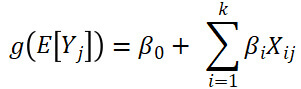
The form of a GLM is
 (1)
(1)
where Yj is the response variable and Xij are factors (also commonly called predictors). Each j index represents a single observation (i.e. one torpedo test). E[Yj] describes the model’s prediction for each observation. The β terms represent model coefficients, where β0 is the intercept and β1,…,βk are the coefficients associated with each factor. Finally, ![]() is the link function, which maps the allowed values of the response variable to the real number line (McCullagh and Nelder 1989). While ordinary linear models generally assume that each term in Yj follows a normal distribution, GLMs allow Yj to be drawn from any exponential-class probability distribution. However, the factors and coefficients can still take any numerical value; therefore, the quantity
is the link function, which maps the allowed values of the response variable to the real number line (McCullagh and Nelder 1989). While ordinary linear models generally assume that each term in Yj follows a normal distribution, GLMs allow Yj to be drawn from any exponential-class probability distribution. However, the factors and coefficients can still take any numerical value; therefore, the quantity ![]() (E[Yj ]) must also be allowed to take any real value.
(E[Yj ]) must also be allowed to take any real value.
The utility of the link function is evident when considering logistic regression, where the response variable is binary (0 or 1) and the quantity E[Yj ] represents the probability the response takes a value of 1 (for example, the probability that a torpedo hits its target). Because probabilities are constrained to fall between 0 and 1, the link function must map quantities from this range to the entire real number line. By convention, the logit function is chosen for binary responses: ![]() (E[Yj ]) =
(E[Yj ]) = ![]() (James, et al. 2013). The link function for an ordinary linear model that follows the normal distribution is always the identity function, which does not transform the response variable.
(James, et al. 2013). The link function for an ordinary linear model that follows the normal distribution is always the identity function, which does not transform the response variable.
Both ordinary and generalized linear models allow factors to be either numeric or categorical. When categorical variables are present, one level of each variable serves as the base case and is included in the intercept term when using treatment coding1. The remaining levels are assigned to discrete Xij terms that take values of 0 or 1 for each observation in the dataset. Each level has its own coefficient βi. For example, “weapon type” could be a categorical factor with levels of “APB 4” and “APB 5.” The “APB 4” level would be absorbed into the intercept term, and “APB 5” would have its own coefficient:
![]() (2)
(2)
For all GLMs, the coefficients β0,…,βk are determined via maximum likelihood estimates (MLEs)2. Because most maximum likelihood estimators are asymptotically normal,3 the coefficient estimates approximately follow a normal distribution when the number of observations is sufficiently large. This allows us to determine the statistical significance of our test statistic, as described below.
Wald Tests
Abraham Wald originally proposed the Wald test as a multiparametric hypothesis test (1943). It determines whether one or more observations agree with what is expected by calculating the squared distance between the observed data and its expected value, normalized by the variance. We give the most general form of the null and alternative hypothesis; here, θ represents the true parameter and θ0 is the parameter value if the null hypothesis is true.
H0:θ = θ0(3.a)
HA:θ ≠ θ0(3.b)
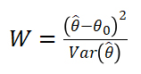
For testing a single hypothesis on a single parameter, the Wald test statistic is:
 (4)
(4)
Here, ![]() is a maximum likelihood estimator for θ. If
is a maximum likelihood estimator for θ. If ![]() follows the normal distribution, follows the chi-squared distribution and the p-values of the statistic can be determined. If the null hypothesis is true, the value of the Wald statistic will be zero. If the observations differ significantly from the hypothesized values, the value of the test statistic will be large and the test will reject the null hypothesis.
follows the normal distribution, follows the chi-squared distribution and the p-values of the statistic can be determined. If the null hypothesis is true, the value of the Wald statistic will be zero. If the observations differ significantly from the hypothesized values, the value of the test statistic will be large and the test will reject the null hypothesis.
This formulation is valid when testing one hypothesis on one parameter. However, our test should compare every model coefficient in the GLM estimated from the ECWAF data with its counterpart in the in-water GLM. Therefore, we must consider the form of the Wald statistic that allows for testing a vector of hypotheses with multiple parameters. Instead of comparing one estimator ![]() to an expected value θ0, we compare the coefficients from two GLMs, both of which are maximum likelihood estimators.4 The modified test statistic is (Harrell 2015):
to an expected value θ0, we compare the coefficients from two GLMs, both of which are maximum likelihood estimators.4 The modified test statistic is (Harrell 2015):
![]() (5)
(5)
Here, V estimates the covariance matrix of the parameter estimates. This calculation assumes that the two GLMs have identical factors and factor levels. If this assumption is met, the value of can be computed by adding the covariance matrices from both GLMs; this procedure is robust to systematic differences in the respective covariance matrices of the two models’ parameter estimates.5 If the models do not have identical factors, the coefficients and covariance matrices should be transformed before calculating the test statistic.
Alternatively, if we assume that the covariance matrices would be identical under the null hypothesis, we would estimate the covariance matrix from the combined set of live data and simulation outputs. The pooled model approach is more sensitive to differences in not only the means, but also the variances of the two models. This approach yields a score-type test rather than a Wald-type test because it uses a covariance matrix estimate consistent under the null hypothesis of model agreement. While this paper focuses on the Wald-type test, we describe both approaches when discussing the statistical details of the test.
Both coefficient estimators are asymptotically normally distributed, which means the test statistic follows an approximate chi-squared distribution with degrees of freedom equal to the number of pairs of parameters. Therefore, just as in the single-parameter case, the statistic’s p-values can be found. However, the test relies on large sample arguments; if the sample size is small in either sample, relative to the number of terms in the model, the test may not perform well. The minimum acceptable sample size depends on many circumstances, including the distribution of the response and the correlation among factors.
This procedure relies on the quality of the estimated statistical models. If the statistical models have problems due to misspecification, low sample size, or other issues, neither the Wald test nor the score test will overcome those problems. Hence, one needs confidence in the estimated models and the correctness of their associated error estimates to use the Wald test or score test. For example, including all torpedo variants’ data in one statistical model would likely fail to produce a credible statistical model due to large differences between variant behavior and testing conditions. These differences may be difficult to accommodate in a linear model without many interaction terms, which eliminates the benefit of including that data in one model.
Test Construction
Applying the Wald Test to M&S and Live Test Data
For the specific case of comparing two GLMs, we asserted that the null hypothesis is true if all of the coefficients in the simulated model are identical to those in the live data model. To test this hypothesis, we calculate the Wald test statistic and associated p-value.
In R, both the lm and glm functions provide a vector of the estimated model coefficients ![]() and
and ![]() . R also includes a function, vcov, that calculates covariance matrices for parameter estimates from a given statistical model. Applying this function to both GLMs and adding the results calculates V. After performing the matrix multiplication shown in equation , we obtain a test statistic that approximately follows a chi-squared distribution with one degree of freedom for each pair of coefficients. We use the calculated test statistic and degrees of freedom to obtain a p-value and determine whether any statistically significant differences between the two GLMs exist.
. R also includes a function, vcov, that calculates covariance matrices for parameter estimates from a given statistical model. Applying this function to both GLMs and adding the results calculates V. After performing the matrix multiplication shown in equation , we obtain a test statistic that approximately follows a chi-squared distribution with one degree of freedom for each pair of coefficients. We use the calculated test statistic and degrees of freedom to obtain a p-value and determine whether any statistically significant differences between the two GLMs exist.
Addressing Inestimable Variable in One or Both Samples
The general calculation of the test statistic is valid for any two GLMs whose factors are identical. However, in many cases, factors or categorical factor levels will be missing or otherwise inestimable in one model. These inestimable factor effects will not have corresponding coefficients in the GLM. For example, the available set of ECWAF data includes results for both the APB 4 and the APB 5 torpedoes. A model created on this dataset includes a coefficient for one of the software variants, while the other one will be absorbed into the intercept. (If there is no explicit intercept term because of a coding scheme for categorical variables, the method creates one when it fixes a factor.) However, because the in-water test data only includes APB 5 torpedoes, its corresponding model will not include any coefficients that describe the torpedo type.
We could have addressed the problem of mismatched coefficients by restricting both models’ factors to the set of factors that are present and estimable in both datasets. However, this solution is not ideal, as it necessitates the loss of useful data and likely results in a less accurate model. In the case of the ECWAF data, omitting all of the APB 4 simulations would exclude a substantial fraction of the available data. Therefore, we constructed our statistical test in a way that would allow the majority of mismatched factors to be retained.
Linear models created using treatment coding (the default coding in R) handle categorical variables by designating one level as the baseline. The baseline levels are included in the model’s intercept, which represents the model’s prediction for an observation where all categorical factors are equal to the baseline level and all numeric factors are 0. The remaining categorical factor levels are treated as separate binary input variables and receive their own coefficients, which represent the change in the model’s prediction relative to the base case. Because the levels in each factor are mutually exclusive, the baseline case includes not only the level defined as the base, but also all other levels that may exist but are not terms in the linear model. Before computing our Wald statistic, we identify all coefficients associated with categorical levels that are present in one model’s dataset but not the other. We then add each level’s coefficient to the corresponding model’s intercept and drop all coefficients associated with other levels of the same factor. After applying this transformation to both models as appropriate, we obtain two models whose coefficients are mathematically comparable.
A similar reasoning applies to numeric factors that are fixed in one model but varied in the other. However, in this case, the coefficient represents the change in the model’s prediction for each unit increase in the factor. Therefore, the numeric coefficients associated with factors that are varied in the first model and fixed in the second must be multiplied by the second dataset’s fixed value before being added to the intercept.
As an example, consider the two models estimated from live torpedo test data and ECWAF data. Suppose that the live test data includes torpedo tests conducted with the APB 5 variant at a variety of depths. The ECWAF data includes the APB 4 and APB 5 variants at the same range of depths. The GLM estimated from the live data is
![]()
The analogous GLM for the model estimated from ECWAF data is

The live model’s intercept term ![]() represents the model’s prediction for the APB 5 variant at a depth of 0. However, the intercept term in the ECWAF model represents that model’s predictions for the APB 4 variant. To obtain a comparable model that describes only APB 5 torpedoes, we must adjust the intercept term. The modified ECWAF model is
represents the model’s prediction for the APB 5 variant at a depth of 0. However, the intercept term in the ECWAF model represents that model’s predictions for the APB 4 variant. To obtain a comparable model that describes only APB 5 torpedoes, we must adjust the intercept term. The modified ECWAF model is
![]()
Now, the model’s intercept term represents the prediction for the APB 5 variant at a depth of 0, just as we see in the live model. We can now run the Wald test to compare the original live test model with the modified ECWAF model.
For VV&A purposes, if the null hypothesis is not rejected—which may lead to the M&S environment being accredited for use in operational testing—it should only be accredited for situations common to both the live data and the M&S outputs. For example, not rejecting the null hypothesis of agreement when APB 4 torpedoes are not present in the live data would, at best, justify accreditation for APB 5 torpedoes only. The limitation to accreditation resulting from having no APB 4 torpedoes in the live test data will always remain.
Statistical Details
In this section we provide a detailed description of the test’s implementation. This section can be skipped by readers who do not need that level of detail.
We use a matrix transformation, which multiplies each coefficient with the corresponding fixed factor setting and adds the product to the intercept term, to make the statistical models comparable. The matrix transformation computes a linear model that fixes a factor and makes predictions with that setting, allowing other factors to vary. In our use case, the transformation takes a GLM that makes predictions for either APB 4 or APB 5 weapons and produces a GLM that makes predictions only for APB 5 weapons.
Suppose that the first l coefficients of ![]() , a vector of length l + k + 1, need to be combined with the simulation statistical model’s intercept coefficient, and the first m coefficients of
, a vector of length l + k + 1, need to be combined with the simulation statistical model’s intercept coefficient, and the first m coefficients of ![]() , a vector of length m + k + 1, need to be combined with the live data statistical model’s intercept. The remaining k coefficients correspond to factors common to both statistical models; under this construct,
, a vector of length m + k + 1, need to be combined with the live data statistical model’s intercept. The remaining k coefficients correspond to factors common to both statistical models; under this construct, ![]() and
and ![]() may differ in length, and thus may not be comparable. The vector
may differ in length, and thus may not be comparable. The vector ![]() contains all the fixed factor settings for the simulation data and
contains all the fixed factor settings for the simulation data and ![]() contains the fixed factor settings for the live data. The length of
contains the fixed factor settings for the live data. The length of ![]() is l and the length of
is l and the length of ![]() is m .
is m .
In our data set, ![]() was an empty vector (thus l = 0), since every factor in the live data’s GLM was also varied in the simulation data.
was an empty vector (thus l = 0), since every factor in the live data’s GLM was also varied in the simulation data. ![]() was a vector of length one (m = 1), since the weapon type was not varied in the live data. This indicated that the coefficient for the weapon dummy variable needed to be added to the intercept.
was a vector of length one (m = 1), since the weapon type was not varied in the live data. This indicated that the coefficient for the weapon dummy variable needed to be added to the intercept.
Let Ik be the identity matrix with dimensions k x k. Then the transformation matrices, written using block matrix notation, are
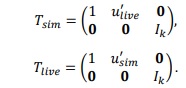
Notice that ![]() is a (k + 1) x (k + l + 1)-dimensional matrix and
is a (k + 1) x (k + l + 1)-dimensional matrix and ![]() is a (k + 1) x (k + m + 1)-dimensional matrix; the block matrices (filled with zeros) have appropriate dimensions to ensure the matrices
is a (k + 1) x (k + m + 1)-dimensional matrix; the block matrices (filled with zeros) have appropriate dimensions to ensure the matrices ![]() and
and ![]() are properly formed.
are properly formed.
Instead of comparing ![]() and
and ![]() , we compare
, we compare ![]() , changing (4) to
, changing (4) to
![]()
When doing so, we need to adjust V’s computation. Since ![]() and
and ![]() , we can use
, we can use
![]()
if we do not use pooled estimators. (We do not describe ![]() or
or ![]() since these are often computed by software using methods described in DasGupta (2008) and Seber and Lee (2003).)
since these are often computed by software using methods described in DasGupta (2008) and Seber and Lee (2003).)
If we use the pooled model’s covariance matrix, we need to use a different set of transformation vectors to compute the correct covariance matrix since there may be factors estimable in the pooled model but not in the individual samples. Suppose ![]() and
and ![]() are vectors of common length p containing the settings for factors that are estimable in the pooled data set but not in the individual data sets. Assume that among the factors appearing in the pooled model, the first l are factors not varied in the simulation, the next m are factors not varied in the live data, the next p are varied in the pooled sample but not in the individual samples, and the remaining k factors are varied in all samples; if
are vectors of common length p containing the settings for factors that are estimable in the pooled data set but not in the individual data sets. Assume that among the factors appearing in the pooled model, the first l are factors not varied in the simulation, the next m are factors not varied in the live data, the next p are varied in the pooled sample but not in the individual samples, and the remaining k factors are varied in all samples; if ![]() represents this model, then it is a (k + l + m + p + 1)-dimensional model. The transformation matrices for the pooled model are
represents this model, then it is a (k + l + m + p + 1)-dimensional model. The transformation matrices for the pooled model are
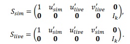
We can interpret ![]() and
and ![]() (both (k + 1) x (k + l + m + p + 1)-dimensional matrices) as allowing for comparison between the pooled model coefficients and the respective models estimated from the simulated and live data samples. Specifically,
(both (k + 1) x (k + l + m + p + 1)-dimensional matrices) as allowing for comparison between the pooled model coefficients and the respective models estimated from the simulated and live data samples. Specifically, ![]()
![]() and
and ![]()
![]() are comparable, as are
are comparable, as are ![]()
![]() and
and ![]()
![]() . If
. If ![]() is the number of simulated runs and
is the number of simulated runs and ![]() the number of live runs, there are
the number of live runs, there are ![]() +
+ ![]() runs used to estimate
runs used to estimate ![]() . The pooled covariance matrix estimator is then
. The pooled covariance matrix estimator is then
![]()
The additional factors involving sample sizes correct for the mismatch in the number of observations used for estimating ![]() and the number of observations used for estimating
and the number of observations used for estimating ![]() and
and ![]() (
(![]() is estimated more precisely than the other linear models and thus has smaller standard errors). If the null hypothesis is true, then W follows a chi-square distribution with k + 1 degrees of freedom when the sample sizes are large, a fact following directly from well-known weak convergence results in probability theory (DasGupta 2008, Seber and Lee 2003, Billingsley 1968).
is estimated more precisely than the other linear models and thus has smaller standard errors). If the null hypothesis is true, then W follows a chi-square distribution with k + 1 degrees of freedom when the sample sizes are large, a fact following directly from well-known weak convergence results in probability theory (DasGupta 2008, Seber and Lee 2003, Billingsley 1968).
Power Study
Here we present results from a Monte Carlo power study. We consider a study with two categorical factors and two continuous factors. One categorical variable has three levels and the other has two levels. One continuous factor ranges from one to ten, the other from -1 to +1. The response variable depends on the factors via a linear model that includes only main effects and an intercept term. If the null hypothesis is true, all of the coefficients of both of the linear models are 0.1; if the alternative hypothesis is true, the all of the coefficients of the model generating the live data are 0.2. Given the small magnitude of the difference between the two linear models, we do not expect high power except in large sample sizes. We use a D-optimal design when generating responses for the live sample. For the simulation sample, we consider both D-optimal designs and full factorial sliced Latin hypersquare designs, a space-filling design (SFD). In the simulation study, we compare the Wald-type test and the score-type test, rejecting the null hypothesis using a α = 0.1 significance level. Both of these tests are asymptotic tests, so we consider a moderate sample size study with 60 live runs and 90 simulation outputs, and a large sample size study with 400 live runs and 600 simulation outputs. We generated 1000 Monte Carlo samples per scenario when estimating power.
In our first case study, the response variable is binary and the data analyzed via logistic regression using the Firth correction (Firth 1993). Note that in instances where the M&S design is a SFD, the assumption of equal covariance matrices under the null hypothesis—used by the score test’s pooled covariance matrix estimate—is false. Also, note that the ideal power for any test when the null hypothesis is true is α = 0.1; we do not want significant deviations from that number. We show the results in Table 1. Both tests do well in the large sample setting. The Wald-type test has poor power in the small sample setting, perhaps due to being unable to maintain the specified Type I error rate (the probability of rejecting a correct null hypothesis) of α = 0.1. The score-type test using a pooled covariance matrix performs better, albeit with a small increase in the Type I error rate. However, while the Wald-type test will eventually obtain the correct Type I error rate and full power, the score-type test may not be able to correct the problem even in large sample sizes.
| M&S Design | True Hypothesis | Wald-Type Test Power | Score-Type Test Power | ||
| D-optimal | Null | 90 | 60 | 0.054 | 0.126 |
| D-optimal | Alternative | 90 | 60 | 0.103 | 0.434 |
| SFD | Null | 90 | 60 | 0.048 | 0.123 |
| SFD | Alternative | 90 | 60 | 0.115 | 0.428 |
| SFD | Null | 600 | 400 | 0.094 | 0.110 |
| SFD | Alternative | 600 | 400 | 0.984 | 0.988 |
Table 1: Power estimates for binomial response variables analyzed with Firth-corrected logistic regression.
We illustrate this potential problem with the score-type test by considering a normally distributed response variable in Table 2. We use D-optimal designs for both the live data and M&S output designs, but the standard deviation of the response is 1 in the M&S outputs and 10 in the live data. Because the standard deviation is 100 times larger than the shift in the coefficients for the fictitious live data samples, detecting the difference in the linear models may be very difficult even with large sample sizes. Low power should not be surprising. The score-type test suffers significant Type I error inflation, driving its higher power in the smaller sample sizes. Importantly, this feature does not disappear in large sample sizes. While the Wald-type test has some Type I error inflation and weaker power in the smaller sample, the Type I error is closer to the nominal rate. With the large sample size, the Type 1 error is at the nominal rate and the test has some power.
| True Hypothesis | Wald-Type Test Power | Score-Type Test Power | ||
| Null | 90 | 60 | 0.121 | 0.320 |
| Alternative | 90 | 60 | 0.160 | 0.361 |
| Null | 600 | 400 | 0.101 | 0.317 |
| Alternative | 600 | 400 | 0.320 | 0.606 |
Table 2: Power estimates for normal response variables analyzed with ordinary least-squares regression
The results for the score-type test seen in Table 2 may be desirable if we desire detecting any difference between M&S outputs and live data, including differences in the variance. However, these differences can emerge for reasons unrelated to M&S quality, such as uncontrolled factors in live testing. Differences in experimental design may also result in the assumption of equal covariance matrices being automatically wrong. Ultimately, the study context will dictate the optimal approach.
While we do not provide exact calculations of power when handling inestimable factors, we can predict the power’s character. If factors need to be combined with the intercept, changes between M&S outputs and live data may confound in a way that obscures the effects of individual factors. These differences may be detected as part of a more comprehensive study in which more factors are varied. However, in the absence of more data, fixed factors should generate a limitation to accreditation, since the resultant GLM will lack predictive power for any fixed factors.
Conclusion
One element of the VV&A process should confirm that the model or simulation produces results similar to the live test data. To that end, we created a statistical test that compares the coefficients of two linear models created on simulated and live data. Because this test was created without specifically referencing the ECWAF data, other VV&A practitioners can use it to conduct further analyses on other M&S tools. Furthermore, its included functionality allows for flexible and statistically rigorous use.
Table of Mathematical Notation
| Notation | Meaning |
| Link function in a generalized linear model (GLM) | |
| βi | A coefficient in a GLM |
| Vectors of coefficient estimates (including the intercept) from simulation, live, and pooled samples, respectively | |
| V | Covariance matrix of relevant parameter estimates |
| E[Yj ] | Expected value, or population mean, of Yj; see any probability textbook for the definition of expected values. In the case of logistic regression for torpedo effectiveness, this is the probability the torpedo hits its target |
| x‘ | Transpose of vector or matrix x |
| θ | Parameter of a probability model |
| θ0 | Value of a parameter of a probability model if the null hypothesis is true |
| Estimate of parameter θ | |
| H0 | Null hypothesis of a statistical test |
| HA | Alternative hypothesis of a statistical test |
| W | Test statistic |
| Var( |
Variance of |
| Var( |
Covariance matrix of live |
| Yj | The jth response variable (for example, a binary variable that is 1 when a torpedo hits its target) |
| Xij | Factor i of run j |
| Transformation matrices to make |
|
| Transformation matrices for properly transforming the pooled covariance matrix | |
| Vectors of length l and m respectively containing factor settings fixed in the named data set but varied in the other | |
| Vectors of length p containing factor settings not varied within the individual data sets but differ between the two | |
| Sample sizes for simulation outputs and live data |
Acknowledgements
We thank various staff members at IDA, including Dr. Steve Rabinowitz, Dr. Elliot Bartis, Dr. John Haman, Dr. Keyla Pagan-Rivera, Dr. Tyler Morgan-Wall, and Dr. Yosef Razin, for their inputs to improve this paper and its description of the ECWAF and its history, along with improvements to presentation and methodology. We also thank anonymous reviewers for their recommended improvements.
References
Billingsley, Patrick. 1968. Convergence of Probability Measures. 1. New York: John Wiley and Sons.
DasGupta, Anirban. 2008. Asymptotic Theory of Statistics and Probability. New York: Springer.
Director, Operational Test and Evaluation. 2019. FY 2019 Annual Report. Washington: Department of Defense. https://www.dote.osd.mil/Annual-Reports/2019-Annual-Report/.
Firth, David. 1993. “Bias reduction of maximum likelihood estimates.” Biometrika 80 (1): 27-38. doi:10.1080/00031305.2021.2023633.
Harrell, Frank E. 2015. Regression Modeling Strategies. 2. New York: Springer.
James, Gareth, Daniela Witten, Trevor Hastie, and Robert Tibshirani. 2013. An Introduction to Statistical Learning with Applications in R. New York: Springer.
McCullagh, Peter, and John A. Nelder. 1989. Generalized Linear Models. 2. Boca Raton: Chapman and Hall.
Seber, George A. F., and Alan J. Lee. 2003. Linear Regression Analysis. Hoboken: John Wiley & Sons.
Wald, Abraham. 1943. “Tests of Statistical Hypotheses Concerning Several Parameters When the Number of Observations Is Large.” Transactions of the American Mathematical Society 54 (3): 426-482.
Endnotes
1 Alternative coding schemes could be used, such as contrast coding. While we do not discuss this issue in depth, the results do not depend on the coding choice. If for any reason (including coding scheme) the linear model lacks an intercept term, matrix transformations effectively create an intercept.
2 This statement is not true in the case of Bayesian models. However, a discussion of Bayesian methodology is beyond the scope of this paper.
3 There are some instances in which an MLE is not asymptotically normal, but a discussion is beyond the scope of this paper. For the use case presented here, asymptotic normality can be assumed.
4 To connect the notation between (3) and (4), ![]()
5 Differing covariance matrices resembles the Behrens-Fisher problem, and our approach to the problem is to use a large sample approximation for the test statistic. We do not attempt in this paper to obtain a more exact distribution.
Author Biographies
Carrington Metts is a Data Science Fellow at IDA. She has a Masters of Science in Business Analytics from the College of William and Mary. Her work at IDA encompasses a wide range of topics, including wargaming, modeling and simulation, natural language processing, and statistical analyses.
Dr. Curtis Miller is a research staff member of the Operational Evaluation Division at the Institute for Defense Analyses. In that role, he advises analysts on effective use of statistical techniques, especially pertaining to modeling and simulation activities and U.S. Navy operational test and evaluation efforts, for the division’s primary sponsor, the Director of Operational Test and Evaluation. He obtained a PhD in mathematics from the University of Utah.